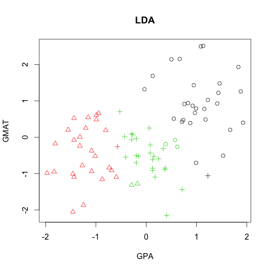
- Linear discriminant analysis (LDA)
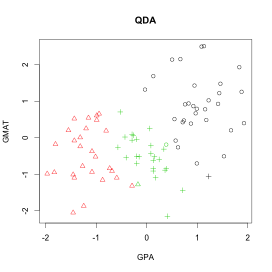
- Quadratic discriminant analysis (QDA)
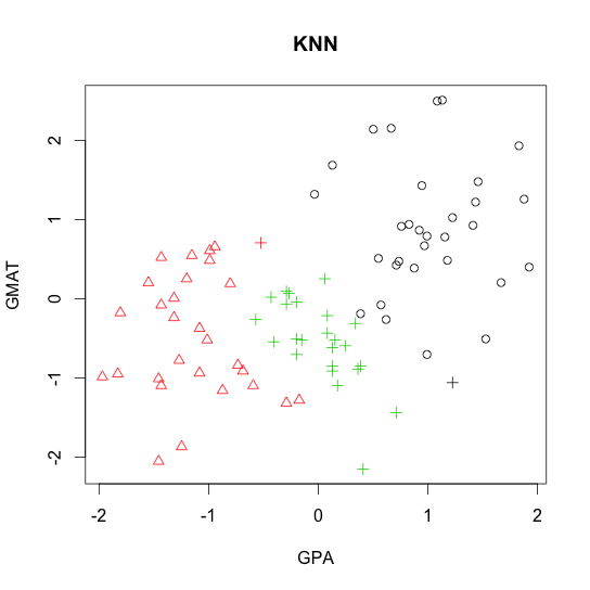
- k-nearest neighbor (KNN)
1 2 3 4 5 6 7 8 9 10 11 12 13 14 15 16 17 18 19 | |
1 2 3 4 5 6 7 8 | |
1 2 3 4 5 6 7 8 9 10 11 12 13 14 15 16 17 18 19 | |
1 2 3 4 5 6 7 8 9 10 11 12 13 14 15 16 17 18 19 | |
1 2 3 4 5 6 7 8 | |
1 2 3 4 5 6 7 8 9 10 11 12 13 14 15 16 17 18 19 | |
It includes the ridge (q=2) and lasso (q =1) as special cases.
More technical details can be found here. Below R code demonstrates:
1 2 3 4 5 6 7 8 9 10 11 12 13 14 15 16 17 18 19 20 21 22 23 24 25 26 27 28 29 30 31 32 33 34 35 36 37 38 39 40 41 42 43 44 45 46 47 48 49 50 51 52 53 54 55 56 57 58 59 60 61 62 63 64 65 66 67 68 69 70 71 72 73 74 75 76 77 78 79 80 81 82 83 84 85 86 87 88 89 90 91 92 93 94 95 96 97 98 99 100 101 102 103 104 105 106 107 108 109 110 111 112 113 114 115 116 117 118 119 120 121 122 123 124 125 126 127 128 129 130 131 132 133 134 135 136 137 138 139 140 141 142 143 144 145 146 147 148 149 150 151 152 153 154 155 156 157 | |

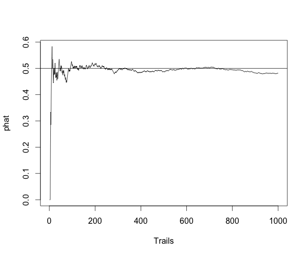
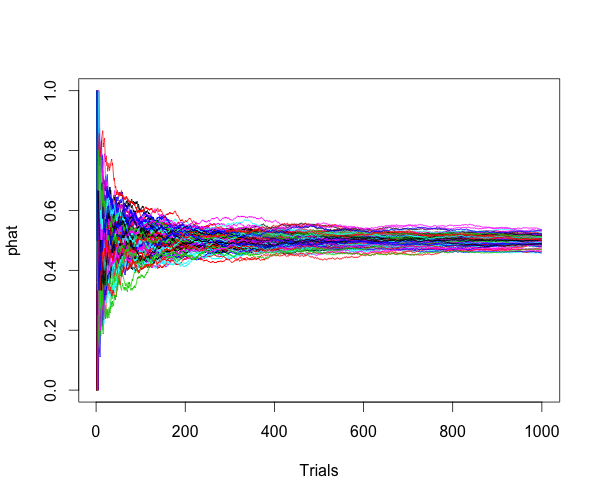
For Bernoulli distribution, $ Y \sim B(n,p) $, $ \hat{p}=Y/n $ is a consistent estimator of $ p $, because:
for any positive number $ \epsilon $.
Here is the simulation to show the estimator is consitent.
1 2 3 4 5 6 7 8 9 | |
1 2 3 4 5 6 7 8 9 10 11 12 13 14 | |
For each replicate,
Individually permute each column of the data matrix.
Conduct the PCA and find the proportion of variance explained by each of the components 1 to s. Store this information.
Repeat 1 and 2 R times.
At the end of this we will have a matrix with R rows and s columns that contains the proportion of variance explained by each component for each replicate.
Finally, compare the observed values from the original data to the set of values from the permutations in order to determine the approximate p-value.
The R code:
1 2 3 4 5 6 7 8 9 10 11 12 13 14 15 16 17 18 19 20 21 22 23 24 25 26 27 28 29 30 31 | |
The result:
$pve
    Comp.1     Comp.2     Comp.3     Comp.4     Comp.5     Comp.6     Comp.7     Comp.8
0.23129378 0.14864525 0.11552865 0.06741744 0.06274641 0.05858431 0.05033795 0.04484122
    Comp.9    Comp.10
0.03873311 0.03431297

$pval
 [1] 0.000 0.000 0.000 1.000 1.000 0.996 1.000 1.000 1.000 1.000
]]>1 2 3 4 5 6 7 8 9 10 11 12 13 14 15 16 17 18 19 20 21 22 23 24 25 | |
1 2 3 4 5 6 7 8 9 10 11 12 13 14 15 16 17 18 19 20 21 22 23 24 25 26 27 28 29 30 31 32 33 34 35 36 37 38 39 40 41 42 43 44 45 46 47 48 49 50 51 52 | |
The probability density function of Gamma distribution is
The MME:
We can calculate the MLE of $ \alpha $ using the Newton-Raphson method.
For $ k =1,2,…,$
where
Use the MME for the initial value of $ \alpha^{(0)} $, and stop the approximation when $ \vert \hat{\alpha}^{(k)}-\hat{\alpha}^{(k-1)} \vert < 0.0000001 $. The MLE of $ \beta $ can be found by $ \hat{\beta} = \bar{X} / \hat{\alpha} $.
Below is the R code.
1 2 3 4 5 6 7 8 9 10 11 12 13 14 15 16 17 18 19 20 21 22 23 24 25 26 27 28 29 30 31 32 33 34 35 36 37 38 39 40 41 42 43 44 45 46 47 48 49 50 51 52 | |
Hopefully, I will write and code more often in 2015.
Stay tuned!
]]>该批产品可通过对孕周12周以上的高危孕妇外周血血浆中的游离基因片段进行基因测序,对胎儿染色体非整倍体疾病21-三体综合征、18-三体综合征和13-三体综合征进行无创产前检查和辅助诊断。
http://www.knowgene.com/question/677 BGISEQ-1000基因测序仪基于Complete Genomics平台,配套的试剂盒为胎儿染色体非整倍体(T21、T18、T13)检测试剂盒(联合探针锚定连接测序法)。CG平台的特点是通量高,但周期较长,因此BGISEQ-1000应该主要会应用于全国范围内的样品,集中测序分析;
BGISEQ-100基因测序仪基于Ion Torrent平台,配套的试剂盒为胎儿染色体非整倍体(T21、T18、T13)检测试剂盒(半导体测序法)。Ion Torrent平台的特点是测序周期短,可灵活部署,BGISEQ-100有很大可能会被部署到有一定业务量的大中型医院,就地采样、测序、分析并出具报告.
]]>总结:科研是聪明且有钱人的游戏。
]]>The book Elements of Statistical Learning (pdf) describes the lasso in detail.
Lasso in R: lars: Least Angle Regression, Lasso and Forward Stagewise, and glmnet: Lasso and elastic-net regularized generalized linear models (Note: lars() function from the lars package is probably much slower than glmnet() from glmnet.)
Adaptive lasso in R
adaptive.lasso function in lqa package (Penalized Likelihood Inference for GLMs)
adalasso function in parcor package (Regularized estimation of partial correlation matrices)
Graphical lasso in R (glasso: Graphical lasso- estimation of Gaussian graphical models)
The joint graphical lasso paper
Joint graphical lasso in R (JGL: Performs the Joint Graphical Lasso for sparse inverse covariance estimation on multiple classes)
]]>One efficient way is using the following recursive formula.
However, the facts are (or would be):
In Statistics Monte Carlo simulation is a “quick” way to compute some complicated formulas. By saying “quick”, I mean I can see the results without knowing or deriving “ugly” Math formulas. It’s actually a very “slow” method in computing aspect.
Anyway, the R function is here.
1 2 3 4 5 6 7 8 9 10 11 12 13 14 15 16 17 18 19 | |
In a small part of my research, I am testing some algorithms to detect co-expression relationship. One way to test algorithm is simulation. In an ideal (simple) case, the expression values of two co-expressed genes can be considered as bivariate normal distributed. To generate expression values of such gene pair or a group of genes given a correlation coefficient, is just to simulate multivariate normal distribution. MASS library in R has an function, mvrnorm, to do that, but it requires a covariance matrix.
The function below is to firstly generate the covariance matrix in order to use the mvnorm function. Because we only know the correlation coefficient, i.e. co-expression relationship (degree), the mean and variance of each gene’s expression profile are random generated in the function. Then the matrix can be calulated as follows.
1 2 3 4 5 6 7 8 9 10 11 12 13 14 15 16 17 18 19 20 21 22 23 24 25 26 27 28 29 30 | |
Please read carefully before using any code or script, and leave a comment if you find some “terrible” error.
Thank you!
[update-2013-08-08] now only perl howto related posts
[update-2015-01-01] All format issues are (putatively) resolved.
]]>The 000wbehost server is good and stable. Most importantly it’s free. Now, I have to transfter to another free and good web hosting service. Github is a good choice. But github does not support wordpress. I tried to transferr the website to github before, but I am not comfortable to write blogs using Markdown.
It’s difficult to find another free service supporting wordpress, and lots of people said the static blogging engine is much better than wordpress. Looks like I will stay here for a while.
]]>(to be continued)
]]>| Name | Machine cost | Read length (bases) | Cost per megabase |
|---|---|---|---|
| Illumina MiSeq | US$125,000 | 500 | 14–70 cents |
| Illumina HiSeq | US$690,000 | 300 | 4–5 cents |
| PacBio RS | US$695,000 | 4,575 | $2–17 |
| Ion Torrent PGM | US$49,000 | 400 | 60 cents–$5 |
| Ion Torrent Proton | US$224,000 | 200 | 1–9 cents |
]]>